How to Master the OVER() Function in SQL: A Step-by-Step Guide to Advanced Data Analysis

Window functions, such as the OVER() clause in SQL, are indispensable tools for elevating data analysis performance. Today, we delve into the intricacies of the OVER() function, unraveling its capabilities and applications in various data scenarios.

Unlike aggregate functions, which group values and can obscure individual data points, window functions excel in precision — they pinpoint specific values while performing aggregations. This unique capability is invaluable in scenarios where detailed, row-level calculations are essential. For instance, consider the task of calculating the average cost price of an item over a year and then determining the deviation of each month’s cost from this average. Here, window functions not only simplify these calculations but also enhance the accuracy of your data analysis.

In this guide, we will explore the practical applications of window functions, particularly focusing on the OVER() clause, and demonstrate how they can transform your approach to SQL data analysis.

Basic OVER() function Syntax:

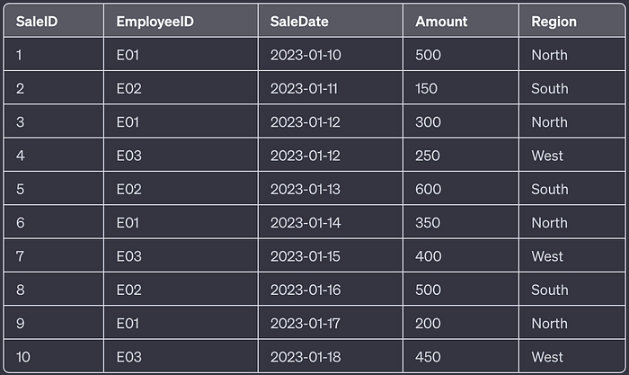
OVER ([PARTITION BY columns] [ORDER BY columns])

Sample Data we will be using throughout the article:

Let’s dive deeper into the components of the OVER() clause and how they shape data analysis in SQL:

Understanding the OVER() clause in SQL involves delving into its key components: ‘PARTITION BY,’ ‘ORDER BY,’ and frame specifications. Each of these elements plays a crucial role in how SQL processes data within a window function

1. PARTITION BY: This clause is used within OVER() to divide the result set into partitions (or groups) of rows. The window function is then applied to each partition independently. The PARTITION BY clause specifies the columns according to which the data is partitioned. Rows that have the same values in the specified columns are grouped into the same partition. If PARTITION BY is not specified, the entire result set is treated as a single partition. In a dataset of sales records, using ‘PARTITION BY StoreID’ will group the data by each store, allowing you to analyze each store’s data independently within the larger dataset.
2. ORDER BY: This clause within OVER() defines the order in which the rows in a partition (or the entire result set, if no PARTITION BY is specified) are processed by the window function. This is crucial for functions where the order of rows is significant, such as running totals or cumulative averages. In a dataset of sales record, using Order By on sales date for each partition will sort the partion values in either ascending or descending order as specified. The default is ascending order.
3. Frame Specification (ROWS/RANGE): In addition to PARTITION BY and ORDER BY, you can further refine the window frame by specifying which rows around the current row should be included in the frame. This is done using the ROWS or RANGE clause. For example, ROWS BETWEEN 1 PRECEDING AND 1 FOLLOWING would define a frame consisting of the current row, the row before it, and the row after it.

Lets see the OVER() function in action:

1. Cumulative Sales Total per region:

SELECT SaleID, EmployeeID, SaleDate, Amount, Region,
       SUM(Amount) OVER(PARTITION BY Region ORDER BY SaleDate) AS CumulativeTotal
FROM SalesData

This query calculates the cumulative total of sales for each region, ordered by the sale date.

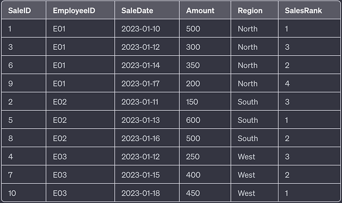
2. Ranking Sales within each region:

SELECT SaleID, EmployeeID, SaleDate, Amount, Region,
       RANK() OVER(PARTITION BY Region ORDER BY Amount DESC) AS SalesRank
FROM SalesData

This query ranks the sales within each region based on the amount, in descending order.

3. Running Total of sales for each employee:

SELECT SaleID, EmployeeID, SaleDate, Amount,
       SUM(Amount) OVER(PARTITION BY EmployeeID ORDER BY SaleDate) AS RunningTotal
FROM SalesData

This query computes the running total of sales for each employee, ordered by the sale date.

A Complex Example

Consider this Scenario: Imagine a company that wants to analyze the performance of its sales team over the past year. The company is interested in not only the total sales per employee but also how each employee’s performance ranks monthly within their region. Additionally, they want to calculate a 3-month moving average for each employee to track performance trends.

SELECT 
    EmployeeID,
    SaleDate,
    Region,
    Amount,
    SUM(Amount) OVER(PARTITION BY EmployeeID) AS TotalSales,
    RANK() OVER(PARTITION BY YEAR(SaleDate), MONTH(SaleDate), 
            Region ORDER BY SUM(Amount) DESC) AS MonthlyRank,
    AVG(Amount) OVER(PARTITION BY EmployeeID ORDER BY
            YEAR(SaleDate), MONTH(SaleDate)ROWS BETWEEN 2 PRECEDING     
            AND CURRENT ROW) AS MovingAvg3Months
FROM 
    SalesData
GROUP BY 
    EmployeeID, SaleDate, Region, Amount

Explanation:

1. Total Sales Per Employee: SUM(Amount) OVER(PARTITION BY EmployeeID) calculates the total sales for each employee across the entire dataset.
2. Monthly Rank Within Region: RANK() OVER(PARTITION BY YEAR(SaleDate), MONTH(SaleDate), Region ORDER BY SUM(Amount) DESC) ranks employees based on their total sales in a given month within their region. This helps in understanding who the top performers are in each region every month.
3. 3-Month Moving Average: AVG(Amount) OVER(PARTITION BY EmployeeID ORDER BY YEAR(SaleDate), MONTH(SaleDate) ROWS BETWEEN 2 PRECEDING AND CURRENT ROW) computes the 3-month moving average of sales for each employee. This window function looks at the current row and the two preceding rows (months) to calculate the average, giving insights into the sales trend for each employee over time.

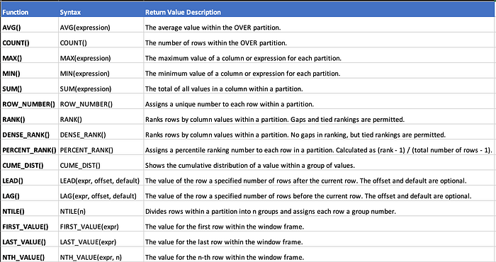
We have only used a couple of window functions. Here is a list of window functions that are very useful:

WINDOW FUNCTIONS

Benefits of Using OVER() in SQL:

1. Efficiency in Data Analysis

The OVER() clause significantly enhances the efficiency of data analysis in SQL. By allowing computations across different partitions of a dataset, it eliminates the need for complex subqueries and multiple queries to achieve the same result. This not only simplifies the code but also reduces the processing time, especially with large datasets.

2. Flexibility

The OVER() clause offers unparalleled flexibility in data analysis. It can be used with a variety of functions like SUM(), AVG(), RANK(), and many others, enabling a wide range of analytical operations. This flexibility allows analysts to easily perform cumulative, moving average, ranking, and window-specific calculations that would be cumbersome without the OVER() clause.

3. Code Readability and Maintenance

The OVER() clause also enhances the readability and maintainability of SQL code. By encapsulating complex calculations within a single, coherent clause, it makes SQL scripts more understandable and easier to modify. This aspect is particularly beneficial in collaborative environments where multiple analysts work on the same codebase.

As we’ve seen, the OVER() clause is a game-changer in SQL, offering remarkable efficiency and flexibility in data analysis. By understanding its concept and key benefits, you can significantly enhance the power and insightfulness of your SQL queries. I encourage you to apply these techniques in your projects and observe the impact firsthand. If you have any experiences or questions, feel free to share — let’s continue learning together. Keep an eye out for my upcoming articles or more deep dives into advanced SQL functionalities.